
Texas Instruments TI-84 Plus Graphics Calculator

Chapter 1 Ingredients of Change: Functions and Linear Models
Models and Functions
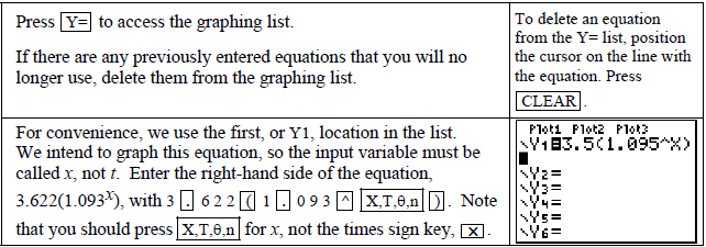
- Graphing a function in an appropriate viewing window is one of the many uses for a function that is entered in the calculator’s graphing list. Because you must enter a function formula on one line, it is important to use parentheses whenever they are needed.
ENTERING AN EQUATION IN THE GRAPHING LIST
- The graphing list contains space for 10 equations, and the output variables are called by the names Y1, Y2, …, and Y0. When you want to graph an equation, you should enter it in the graphing list. You must use X as the input variable if you intend to draw the graph of the equation or use the calculator’s table function. We illustrate graphing with the equation in Example 3 of Section 1.1: v(t) = 3.5(1.095t).
TRACING TO ESTIMATE OUTPUTS
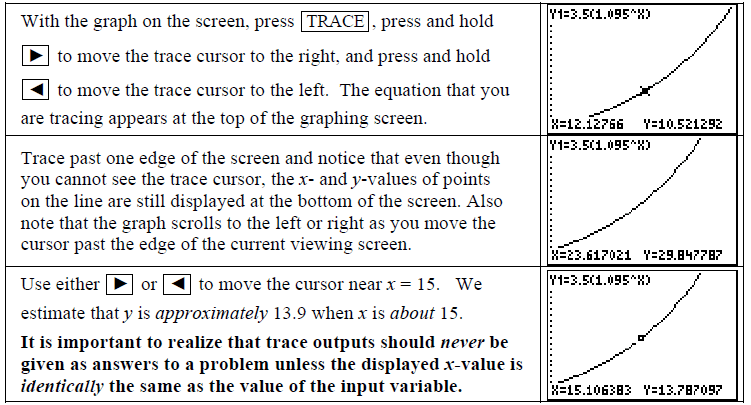
- You can display the coordinates of certain points on the graph by tracing. Unlike the substitution feature of TRACE that was discussed on the previous page, the x-values that you see when tracing the graph depend on the horizontal view that you choose. The output values that are displayed at the bottom of the screen are calculated by substituting the x-values into the equation that is being graphed. We again assume that you have the function v(x) = 3.5(1.095x) entered in the Y1 location of the Y= list.
FINDING INPUT VALUES USING THE SOLVER
- Your calculator solves for the input values of any equation that is in the form “expression = 0”. This means that all terms must be on one side of the equation and 0 must be on the other side before you enter the equation into the calculator. The expression can, but does not have to, use x as the input variable. The calculator offers several methods of solving for input variables. We first illustrate using the SOLVER. (Solving using graphical methods will be discussed after using the SOLVER is explored.) You can refer to an equation that you have already entered in the Y= list or you can enter the equation in the solver.
HAVING THE CALCULATOR ENTER EVENLY SPACED INPUT VALUES
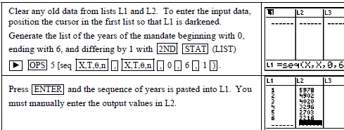
- When an input list consists of many values that are the same distance apart, there is a calculator command that will generate the list so that you do not have to type the values in one by one. The syntax for this sequence command is seq(formula, variable, first value, last value, increment). When entering years that differ by 1, the formula is the same as the variable and the increment is 1. Any letter can be used for the variable we choose to use X. We illustrate the sequence command used to enter the input for the population data in Table 1.17 in Section 1.3 of Calculus Concepts
| Year of mandate | 0 | 1 | 2 | 3 | 4 | 5 | 6 |
| Population | 7290 | 5978 | 4902 | 4020 | 3296 | 2703 | 2216 |
Chapter 2 Describing Change: Rates
- As you calculate average and other rates of change, remember that every numerical answer in a context should be accompanied by units telling how the quantity is measured. You should also be able to interpret each numerical answer. It is only through their interpretations that the results of your calculations will be useful in real-world situations.
FINDING THE AVERAGE RATE OF CHANGE
- Finding an average rate of change using a function is just a matter of evaluating the equation at two different values of the input variable and dividing by the difference of those input values. We illustrate this concept using the function describing the temperature on a typical day in May in a certain Midwestern city that is given in Example 3 of Section 2.1 of Calculus Concepts.

- Recall that the rate of change units are output units per input unit. On average, the temperature on a typical day in May in a certain Midwestern city decreased about 2.4 o F per hour between 11:30 A.M. and 6 P.M

MAGNIFYING A PORTION OF A GRAPH
- The ZOOM menu of your calculator allows you to magnify any portion of a graph. Consider the graph shown in Figure 2.7 in Section 2.2 of Calculus Concepts. The temperature model is T(x) = −0.804×2 + 11.644x + 38.114 degrees Fahrenheit where x is the number of hours after 6 a.m.
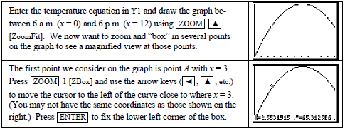
 Reset Xmin to 0, Xmax to 12, and redraw the graph of T with ZoomFit. Repeat the zoom and box steps for point B with x = 7.24 and point C with x = 9. Note for each point how the graph of the parabola looks more like a line the more you magnify the view. These are illustrations of local linearity.
Chapter 3 Determining Change: Derivatives
Exponential and Logarithmic Rate-of-Change Formulas
The calculator only approximates numerical values of slopes – it does not give a slope in formula form. You also need to remember that the CALCULATOR calculates the slope (i.e., the derivative) at a specific input value by a different method than the one we use to calculate the slope.
CALCULATING dy/dx AT SPECIFIC INPUT VALUES
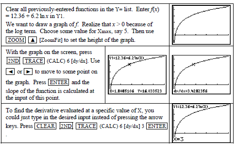
- The previous two sections of this Guide examined the calculator’s numerical derivative nDeriv(f(x), x, a) and illustrated that it gives a good approximation to the slope of the tangent line at points where the instantaneous rate of change exists. You can also evaluate the calculator’s numerical derivative from the graphics screen using the CALC menu. However, instead of being named nDeriv, it is called dy/dx. We illustrate this use with the function in part A of Example 2 in Section 3.3.


The Chain Rule
- You probably noticed that checking your answer for a slope formula graphically is more difficult than checking your answer using the table if you have to spend a lot of time finding a window in which to view the graph. Practice with these methods will help you determine which is the best to use to check your answer.
SUMMARY OF CHECKING METHODS
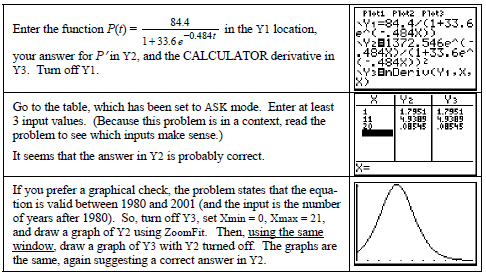
- Before you begin checking your answer, make sure that you have correctly entered the function. It is very frustrating to miss the answer to a problem because you have made an error in entering a function in your calculator. We summarize the methods of checking your algebraic answer using the function in Example 3 of Section 3.4 of Calculus Concepts.
Chapter 4 Analyzing Change: Applications of Derivatives
Relative and Absolute Extreme Points
- Your calculator can be very helpful for checking your analytic work when you find optimal points and points of inflection. When you are not required to show work using derivative formulas or when an approximation to the exact answer is all that is required, it is a simple process to use your calculator to find optimal points and inflection points.
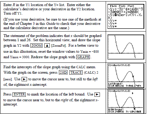
FINDING X-INTERCEPTS OF SLOPE GRAPHS
- Where the graph of a function has a relative maximum or minimum, the slope graph has a horizontal tangent. Where the tangent line is horizontal, the derivative of the function is zero. Thus, finding where the slope graph crosses the input axis is the same as finding the input of a relative extreme point.
- Consider, for example, the model for Acme Cable Company’s revenue for the 26 weeks after it began a sales campaign, where x is the number of weeks since Acme began sales: R(x) = −3×4 + 160×3 – 3000×2 + 24,000x dollars
- In Example 2 of Section 4.2 of Calculus Concepts, we are first asked to determine when Acme’s revenue peaked during the 26-week interval.
Chapter 5 Accumulating Change: Limits of Sums and the Definite Integral
Results of Change and Area Approximations
- So far, we have used the calculator to investigate rates of change. In this chapter, we consider the second main topic in calculus – the accumulation of change. Your calculator has many useful features that will assist in your investigations of the results of change.
AREA APPROXIMATIONS USING LEFT RECTANGLES
- The calculator lists can be used to approximate, using left rectangles, the area between the horizontal axis and a rate of change function between two specified input values. We illustrate the necessary steps using the data for the number of customers entering a large department store during a Saturday sale. These data appear in Table 5.1 of Section 5.1 in Calculus Concepts.
| Hours after 9 A.M. | 0 | 0.75 | 1.25 | 2 | 2.75 | 3.25 | 4.25 | 5.5 | 6.167 | 7 | 8.25 | 9.5 | 10.5 | 11.25 |
| Customers per hour | 60 | 120 | 180 | 240 | 240 | 300 | 300 | 300 | 300 | 240 | 240 | 180 | 120 | 120 |
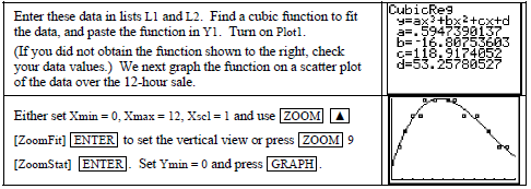
- We want to approximate the area under the cubic graph and above the x-axis during the 12-hour period using rectangles of equal width (1 hour).
 Consider what is now on the lists. L1 contains the left endpoints of the 11 rectangles and L2 contains the heights of the rectangles. If we multiply the heights by the widths of the rectangles (1 hour) and enter this product in L3, we will have the rectangle areas in L3.
 When you use left rectangles to approximate the results of change, the rightmost data point is not the height of a rectangle and is not used in the computation of the left-rectangle area. Similarly, when using right rectangles to approximate the results of change, the leftmost data point is not the height of a rectangle and is not used in the computation of the right-rectangle area.
Chapter 6 Analyzing Accumulated Change: Integrals in Action
Streams in Business and Biology
- You will find your calculator very helpful when dealing with streams that are accumulated over finite intervals. Finding either the future or present value of a continuous income stream is simply finding the value of a definite integral.
DETERMINING THE FLOW-RATE FUNCTION FOR AN INCOME STREAM
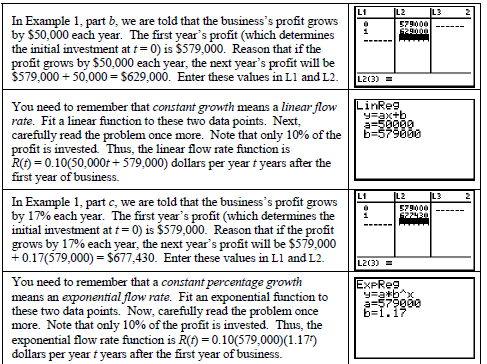
- The calculator can often help you to find the equation for an income stream flow rate. Note that it is not necessary to use the calculator to find such an equation we present this as a technique to use only if you find writing the equation from the word description difficult. We illustrate these ideas as they are given in Example 1 of Section 6.2 of Calculus Concepts.
 CAUTION: If you attempt to draw a scatter plot on the calculator, you will get an error message because the calculator, using the output data in L2, sets Ymin = Ymax. (You need to draw the scatter plot using paper and pencil.) If you want to see the horizontal line graph on the calculator, change Ymin and Ymax so that 57,900 is between the two values and press GRAPH.
Chapter 7 Repetitive Change: Cycles and Trigonometry
FITTING A SINE MODEL TO DATA
- Before fitting any model to data, remember that you should construct a scatter plot of the data and observe what pattern the data appears to follow. Example 1 in Section 7.2 asks you to find a sine model for cyclic data with the hours of daylight on the Arctic Circle as a function of the day of the year on which the hours of daylight are measured. (January 1 is day 1.) These data appear in Table 7.2 of Calculus Concepts.
| Day of the year | -10 | 81.5 | 173 | 264 | 355 | 446.5 | 538 | 629 | 720 | 811.5 |
| Hours of daylight | 0 | 12 | 24 | 12 | 0 | 12 | 24 | 12 | 0 | 12 |
- Clear any old data. Delete any functions in the Y= list and turn on Plot 1. Enter the data in the above table in lists L1 and L2. Construct a scatter plot of the data. When using the sine regression in the calculator, it is sometimes necessary to have an estimate of the period of the data.
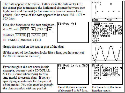
- NOTE: If you do not think the original function the calculator finds fits the data very well, try specifying a period and see if a better-fitting equation results. It didn’t here, but it might be with a different set of data. If you still cannot find an equation, you can tell the calculator how many times to go through the routine that find the equation. This number of iterations is 3 if not specified. The number should be typed before L1 when initially finding the equation.
Chapter 8 Dynamics of Change: Differential Equations and Proportionality
Numerically Estimating by Using Differential Equations: Euler’s Method
- Many of the differential equations we encounter have solutions that can be found by determining an antiderivative of a given rate-of-change function. Thus, many of the techniques that we learned using the calculator’s numerical integration function apply to this chapter.
EULER’S METHOD FOR A DIFFERENTIAL EQUATION WITH ONE INPUT VARIABLE
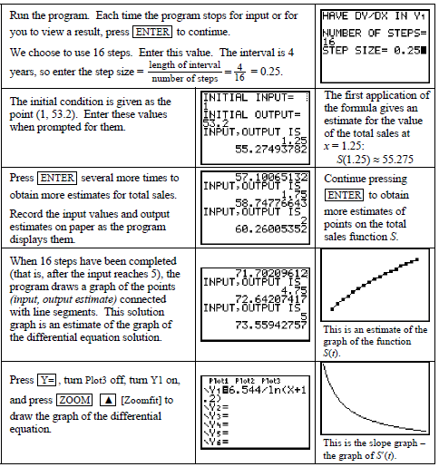
- You may encounter a differential equation that cannot be solved by standard methods and you may need to draw an accumulation graph for a differential equation without first finding an antiderivative. In either of these cases, numerically estimating a solution using Euler’s method is helpful. This method relies on the use of the derivative of a function to approximate the change in that function. Recall from Section 4.1 of Calculus Concepts that the approximate change in a function f at a point is the rate of change of f at that point times a small change in x. That is, f(x + h) – f(x) ≈ f ′ (x).h where h represents the small change in x. Now, if we let b = x + h and x = a, the above expression becomes f(b) – f(a) ≈ f ′ (a).(b – a) or f(b) ≈ f(a) + (b – a).f ′ (a)
- The starting values for the coordinates of the point (a, b) will be given to you and are often called the initial condition. The next step is to repeatedly apply the formula given above to use the slope of the tangent line at x = a to approximate the change in the function between inputs a and b. When h, the distance between a and b, is fairly small, Euler’s method will often give close numerical estimates of points on the solution to the differential equation containing f ′ (x).
- We illustrate Euler’s method for a differential equation containing one input variable with the differential equation in Example 1 of Section 8.3. This equation gives the rate of change of the total sales of a computer product t years after the product was introduced: ds/dt=6.544/ln(t=1.2) billion dollars per year
- Because Euler’s method involves a repetitive process, a program that performs the calculations used to find the approximate change in the function can save you time and eliminate computational errors and some errors in rounding. The download is available at: http://college.hmco.com/mathematics/latorre/calculus_concepts/3e/students/programs.html

Chapter 9 Ingredients of Multivariable Change: Models, Graphs, Rates
FINDING A CROSS-SECTIONAL MODEL FROM DATA (HOLDING THE FIRST INPUT VARIABLE CONSTANT)
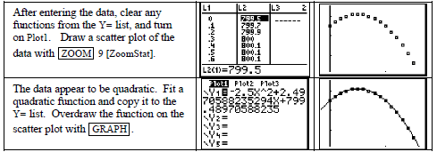
- We are to find the cross-sectional model E(0.8, n) using the elevation data that appears in Table 9.4 of Section 9.2 in Calculus Concepts. However, the data you use in the activities will be obtained from a multivariable table. So we digress for a moment to understand how to find the data you need in such a table.
- Refer to Table 9.3 on page 574 of the text. Remember that “rows” (containing the n data) go from left to right horizontally and “columns” (containing the e data) go from top to bottom vertically. In E(0.8, n), e is constant at 0.8 and n varies. Thus, choose the values for n that appear on the left side of the table (vertically) in L1 and the elevations E in the e = 0.8 column of Table 9.3 in L2. In general, the inputs that you enter in L1 are either across the top or down the left side of the table, and the outputs that you enter in L2 will always be in the main body of any multivariable data table in this text. Thus the data we enter are these values:
| n (miles) | 0 | 0.1 | 0.2 | 0.3 | 0.4 | 0.5 | 0.6 | 0.7 |
| Elevation (feet above sea level) | 799.5 | 799.7 | 799.9 | 800.0 | 800.1 | 800.1 | 800.1 | 800.0 |
| n (miles) | 0.8 | 0.9 | 1.0 | 1.1 | 1.2 | 1.3 | 1.4 | 1.5 |
| Elevation (feet above sea level) | 799.9 | 799.7 | 799.5 | 799.2 | 798.9 | 798.5 | 798.1 | 797.6 |
Chapter 10 Analyzing Multivariable Change: Optimization
FINDING OPTIMAL POINTS USING MATRICES AND CLASSIFYING OPTIMAL POINTS UNDER CONSTRAINED OPTIMIZATION
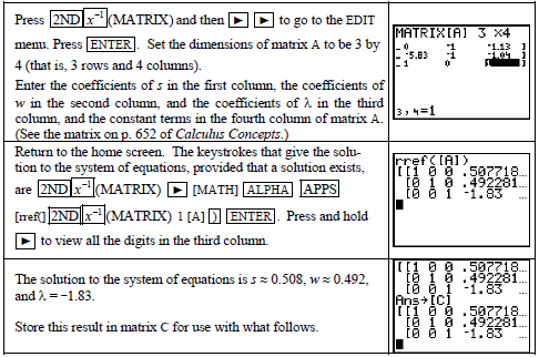
- Remember that a matrix solution method only can be used with a system of linear partial derivative equations. We choose to illustrate the matrix process of solving with matrix Method 2 for the sausage production function in Example 3 of Section 10.3 in Calculus Concepts. The system of partial derivative equations and the constraint, written with the constant terms on the right-hand side of the equations and the coefficients of the three input variables in the same positions on the left-hand side of each equation, is -5.83s – λ = −1.13 -5.83w– λ = −1.04 w+s=1
- When a particular variable does not appear in an equation, its coefficient is zero.

- We will use the solver with Y2 to find values on the constraint to test against the optimal value.
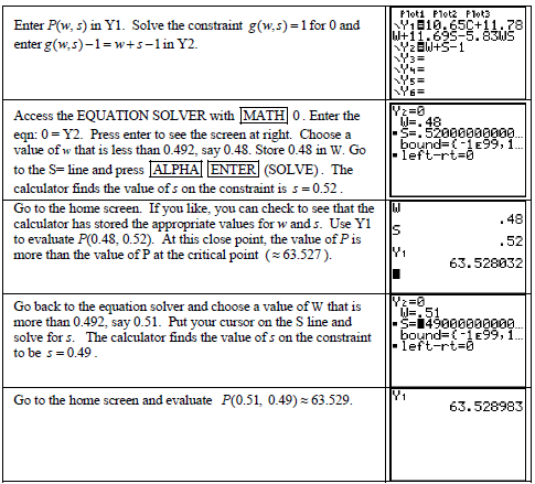
- Because the value of P at the close points is more than its value at the critical point, w ≈ 0.492 whey protein, s ≈ 0.508 skim milk powder, and P ≈ 10.277% cooking loss is a minimum point.
For more Manuals by Texas Instruments, visit ManualsLibraryy
Texas Instruments TI-84 Plus Graphics Calculator-FAQs
How can I view my previous calculations on the TI-84 Plus?
Press the up (↑) and down (↓) arrows on the Home screen to scroll through your calculation history and reuse previous entries or answers.
How do I adjust the brightness on my TI-84 Plus?
Press [2nd], then use the up (▲) arrow to darken or the down (▼) arrow to lighten the screen.
How long does it take to fully charge the TI-84 Plus?
A full charge takes approximately four hours when using a TI wall adapter or a TI Charging Station CE.
Is the TI-84 Plus a scientific calculator?
No, it is a graphing calculator designed for advanced math and science applications, but it includes scientific calculator functions.
How do I calculate the mode of a data set?
The mode is the number that appears most frequently in a data set. Count the occurrences of each number and identify the most common one.
How do I find the maximum or minimum of a function?
Press [2nd] → [CALC] → Choose 3: minimum or 4: maximum. Set left and right bounds using the arrow keys, then press ENTER.
Is the TI-84 Plus rechargeable?
Yes, the TI-84 Plus CE has a rechargeable battery that lasts up to a month on a full charge, depending on usage.
How do I type letters on the TI-84 Plus?
Press [ALPHA] before each letter. To enter multiple letters, press [2nd] [ALPHA] to activate Alpha Lock mode.


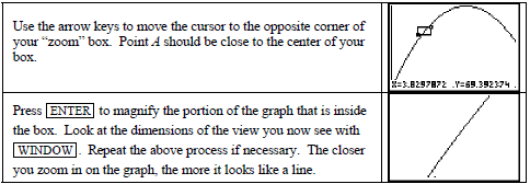 Reset Xmin to 0, Xmax to 12, and redraw the graph of T with ZoomFit. Repeat the zoom and box steps for point B with x = 7.24 and point C with x = 9. Note for each point how the graph of the parabola looks more like a line the more you magnify the view. These are illustrations of local linearity.
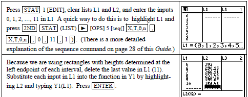 Consider what is now on the lists. L1 contains the left endpoints of the 11 rectangles and L2 contains the heights of the rectangles. If we multiply the heights by the widths of the rectangles (1 hour) and enter this product in L3, we will have the rectangle areas in L3.
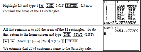 When you use left rectangles to approximate the results of change, the rightmost data point is not the height of a rectangle and is not used in the computation of the left-rectangle area. Similarly, when using right rectangles to approximate the results of change, the leftmost data point is not the height of a rectangle and is not used in the computation of the right-rectangle area.
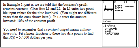 CAUTION: If you attempt to draw a scatter plot on the calculator, you will get an error message because the calculator, using the output data in L2, sets Ymin = Ymax. (You need to draw the scatter plot using paper and pencil.) If you want to see the horizontal line graph on the calculator, change Ymin and Ymax so that 57,900 is between the two values and press GRAPH.